I spent six years building data platforms on Google Cloud. BigQuery was at the centre of almost everything - ingestion, transformation, analytics, cost management. After a while you stop thinking about the tool and start thinking about the problem, which is usually when you discover that the features doing the most work for you are not the ones on the landing page.

These are not obscure features. They are documented, they are stable, and they have been around long enough that there is no excuse for not knowing them. But in my experience working across multiple clients and mentoring junior data engineers and analytics engineers, most people either don't know they exist or don't fully understand when to use them.

So here are three BigQuery features I used constantly in production, why I used them, the specific situations where they saved me, and what I tried to teach juniors when I introduced them.

I am also including a bonus section on partitioning and clustering at the end, because it is impossible to talk about getting the most out of BigQuery without covering those two.

1. Time Travel - my biggest ally on production deploy

BigQuery stores historical versions of your data for up to 7 days by default. You can query any table as it existed at any point within that window using the FOR SYSTEM_TIME AS OF clause. This is called Time Travel.

-- Query a table as it existed 2 hours ago
SELECT *
FROM `project.dataset.orders`
FOR SYSTEM_TIME AS OF TIMESTAMP_SUB(CURRENT_TIMESTAMP(), INTERVAL 2 HOUR);

-- Query using an exact timestamp
SELECT *
FROM `project.dataset.orders`
FOR SYSTEM_TIME AS OF '2026-04-12 09:00:00 UTC';

You can also restore an entire table to a previous state by combining Time Travel with CREATE OR REPLACE TABLE:

-- Restore a table to how it looked 4 hours ago
CREATE OR REPLACE TABLE `project.dataset.orders`
AS SELECT *
FROM `project.dataset.orders`
FOR SYSTEM_TIME AS OF TIMESTAMP_SUB(CURRENT_TIMESTAMP(), INTERVAL 4 HOUR);

Note: The two examples above inquires computing costs. But there's a way to avoid costs and I will explain it below.

How I actually used it

My most common use case was production deploys. When shipping a significant change to a core transformation model - a redefined revenue metric, a reworked customer segmentation, a refactored staging model - I would snapshot the current state of the affected table before running the deploy, then compare the before and after row counts and key aggregations.

If something went wrong, I did not need to restore a backup or replay a pipeline from scratch. I would just query the table as it existed before the deploy, validate what I needed, and restore if necessary. The whole operation took minutes rather than hours.

The other scenario I used it constantly was incident response. When a business stakeholder raised a data discrepancy - "the number was different this morning" - Time Travel let me go back and see exactly what the table contained at the time they were looking at it. No speculation, no "it might have been a refresh issue." Just the actual data, at the actual time.

What I taught juniors

Most engineers I worked with never heard of it, had a background in another cloud provider or worked with databases where point-in-time recovery meant restoring from a backup - a slow, infrastructure-heavy operation you would only do in a real emergency. The mental model was: backups are for disasters, not for everyday mistakes.

Time Travel changes that. It makes point-in-time access fast and cheap enough to use as part of your normal workflow. I would tell juniors: treat Time Travel as your personal undo button for data. Before any deploy that touches a production table, take 30 seconds to note the current timestamp. If anything goes wrong in the next two hours, you have an escape hatch.

The other thing I emphasised: Time Travel has a cost. Querying historical data still uses query compute, and storing historical versions contributes to storage costs. For large tables with frequent updates, it is worth being aware of this.
However.. to avoid query compute, you can use Cloud Shell instead:

-- Base bq copy command:
bq cp dataset_id.table_id@timestamp dataset_destination.table_destination

-- You can set a different project as destination just by adding:
bq cp dataset_id.table_id@timestamp project_id:dataset_destination.table_destination

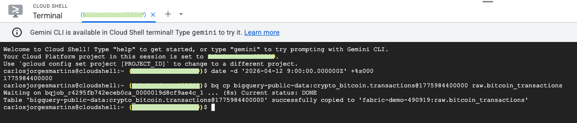
-- Now, to restore a table you need first to determine a UNIX timestamp in milliseconds to point the exact time when the table existed. You can use the Linux date command to generate the timestamp or use https://currentmillis.com/ 
date -d '2026-04-12 9:00:00.000000Z' +%s000

--which returns 1775984400000. And now I can use it like

bq cp mydataset.mytable@1775984400000 mydataset.newtable

Real example:

2. QUALIFY - the window function filter that eliminates subqueries

If you have ever needed to filter the results of a window function, you know the pain. In standard SQL, window functions cannot be referenced in a WHERE clause because they are evaluated after filtering.

So imagine this scenario where you have to pick unique entries by a given column.

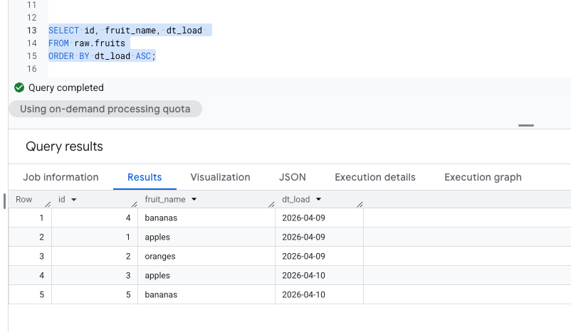
The typical workaround is a subquery or a CTE:

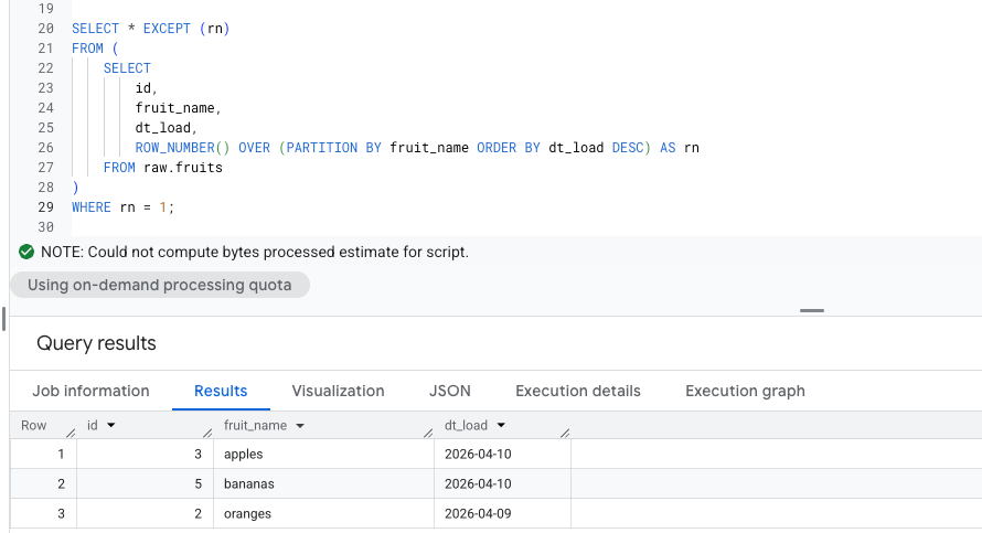
BigQuery supports QUALIFY, which lets you filter on window function results directly in the main query, so no subquery or CTE needed:

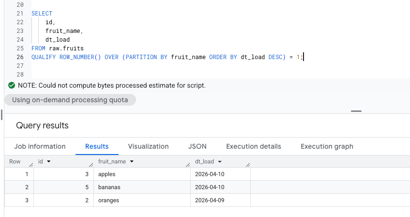
Both queries return the same result. But the QUALIFY version is shorter, easier to read, and avoids nesting.

How I actually used it

Deduplication was the case I reached for QUALIFY most often. In any pipeline that ingests from a source system without guaranteed uniqueness where you inevitably end up with duplicates that need to be resolved before the Silver layer or simply if your ingestion strategy is "append only".

The other common use case was "top N per group" queries - the most recent record per customer, the highest-value order per region, the latest status per transaction. These come up constantly in analytics engineering and the QUALIFY version is significantly cleaner than the nested alternative.

In dbt, QUALIFY fits naturally into staging models where you are doing initial cleaning and deduplication. If you are already filtering on window functions using CTEs, it is worth revisiting those models and simplifying them.

What I taught juniors

The first time most people see QUALIFY they ask two questions: why does this exist, and why doesn't standard SQL support it?

The answer to the first question is practical - window functions in standard SQL are evaluated in the SELECT phase, after WHERE filtering, which means you cannot reference them in WHERE. QUALIFY is BigQuery's (like Snowflake and a few others) solution to this sequencing problem.

The answer to the second question is that QUALIFY is not part of the ANSI SQL standard, which means it does not exist in Postgres, SQL Server, or MySQL. This is important for junior engineers who work across multiple platforms. QUALIFY is a BigQuery and Snowflake feature, not something they can use everywhere.

I always paired the QUALIFY lesson with a broader point: understanding SQL's logical processing order (FROM - WHERE - GROUP BY - HAVING - SELECT - QUALIFY - ORDER BY - LIMIT) is one of the most useful things a data engineer can internalise. A lot of confusing query behaviour makes sense once you understand at which stage each clause runs.

In peer code reviews, this was often the first "issue" I flagged. Cleaning it up leads to significantly cleaner and more maintainable code.

3. INFORMATION_SCHEMA - query your own metadata like a table

Every object in BigQuery (dataset, table, view, job, reservation) has metadata, and that metadata is queryable with SQL through INFORMATION_SCHEMA. You do not need the UI, you do not need the CLI, you do not need a monitoring tool. You just write a query.

The most useful views for day-to-day engineering work:

-- All tables in a dataset with row counts and sizes
SELECT
    table_name,
    row_count,
    ROUND(size_bytes / POW(10,9), 2) AS size_gb,
    creation_time,
    last_modified_time
FROM `project_id`.`region-REGION`.INFORMATION_SCHEMA.TABLE_STORAGE
ORDER BY size_bytes DESC;

-- change region accordingly - for example: region-us

-- Recent query history with costs
SELECT
    job_id,
    user_email,
    query,
    ROUND(total_bytes_processed / POW(10,9), 2) AS gb_processed,
    ROUND(total_bytes_processed / POW(10,12) * 5, 4) AS estimated_cost_usd,
    creation_time,
    total_slot_ms
FROM `region-us.INFORMATION_SCHEMA.JOBS_BY_PROJECT`
WHERE creation_time >= TIMESTAMP_SUB(CURRENT_TIMESTAMP(), INTERVAL 24 HOUR)
    AND job_type = 'QUERY'
    AND state = 'DONE'
ORDER BY total_bytes_processed DESC
LIMIT 20;

-- Find the most expensive queries in the last 7 days
SELECT
    user_email,
    ROUND(SUM(total_bytes_processed) / POW(10,12) * 5, 2) AS total_cost_usd,
    COUNT(*) AS query_count
FROM `region-us.INFORMATION_SCHEMA.JOBS_BY_PROJECT`
WHERE creation_time >= TIMESTAMP_SUB(CURRENT_TIMESTAMP(), INTERVAL 7 DAY)
    AND job_type = 'QUERY'
    AND state = 'DONE'
GROUP BY user_email
ORDER BY total_cost_usd DESC;

A few things worth knowing about INFORMATION_SCHEMA:

• INFORMATION_SCHEMA.JOBS_BY_PROJECT requires the region prefix (e.g. region-eu or region-us). It does not work without it
• The cost calculation above uses the on-demand pricing of $5 per TB processed, so adjust for your actual pricing model
• total_bytes_processed reflects bytes processed before cache. If a query hits cache, it processes 0 bytes and costs nothing

How I actually used it

The scenario I came back to most was onboarding onto a new client project. When you join an existing data platform, one of the first things you want to understand is: what is expensive, what is growing fast, and who is running what. INFORMATION_SCHEMA answers all three questions in a few queries, without needing anyone to give you a walkthrough of the UI or read you a list of tables.

The other place it became part of my workflow was before any significant refactoring job. Before touching a model that feeds multiple downstream consumers, I would query INFORMATION_SCHEMA.VIEWS to find all views that reference it, and INFORMATION_SCHEMA.TABLE_STORAGE to understand whether the table was large enough that the refactor would have meaningful cost implications. It is the kind of due diligence that takes 5 minutes and saves hours.

What I taught juniors

The INFORMATION_SCHEMA "lesson" was usually part of a broader conversation about ownership. A data engineer who understands what is happening in their platform: what is expensive, what is growing, where the slow queries are, is fundamentally different from one who waits to be told there is a problem.

I would set juniors a challenge: using only INFORMATION_SCHEMA queries, tell me the three most expensive queries run on this project in the last week, who ran them, and what they were doing. It forces them to explore the metadata views, understand the schema, and start thinking about cost as part of their normal awareness (not just as something for the FinOps team to worry about).

The other thing I emphasised: INFORMATION_SCHEMA is your audit trail. If a table gets accidentally overwritten, if a cost spike appears out of nowhere, if someone asks "who changed this and when" the answers are in INFORMATION_SCHEMA.JOBS.

My point is: get comfortable querying it before you need it urgently.

Bonus - Partitioning and Clustering

These are not hidden gems, they are well documented and widely discussed. But I am including them here because they are so often misunderstood or misapplied in practice, and because the combination of the two is more powerful than either alone.

Partitioning

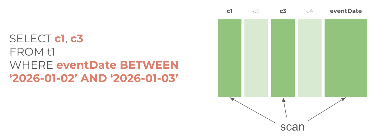
Partitioning divides a table into segments based on the values in a column, typically a date or timestamp. When you query with a filter on the partition column, BigQuery reads only the relevant partitions rather than scanning the full table. This reduces both cost and query time.

Now the same table but partitioned by eventDate:

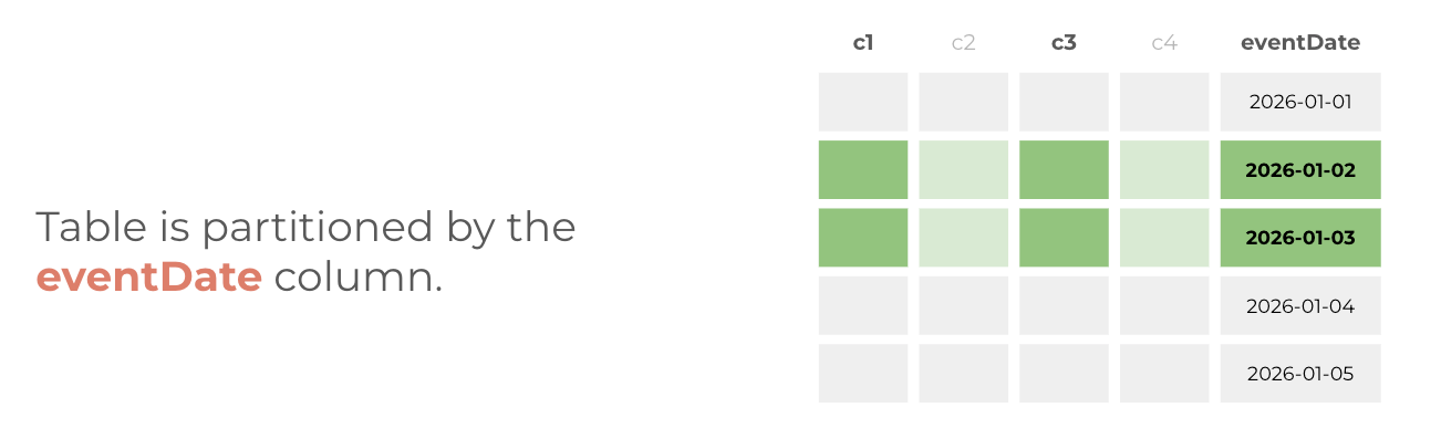
In this case, the table was segmented by a particular column so you could improve query performance and control costs by reducing the number of bytes read by the query.

Example to partition a table in BigQuery:

-- Create a partitioned table
CREATE TABLE `project.dataset.events`
PARTITION BY DATE(event_timestamp)
AS SELECT * FROM `project.dataset.events_raw`;

-- This query scans only the March 2026 partition
SELECT *
FROM `project.dataset.events`
WHERE DATE(event_timestamp) BETWEEN '2026-03-01' AND '2026-03-31';

The most common mistake I saw with partitioning: choosing a partition column that does not match how the table is actually queried. If analysts always filter on order_date but you partition on created_at, most queries still scan the full table. Talk to whoever queries the data before deciding how to partition it.

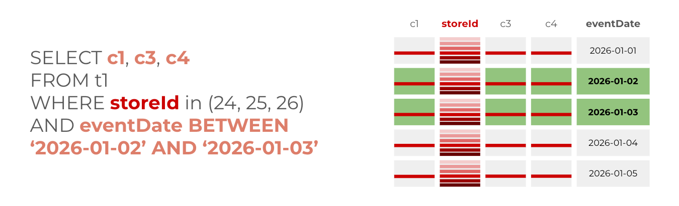
Clustering

Clustering sorts data within partitions based on one or more columns. When you query with a filter on a clustered column, BigQuery scans only the relevant sorted blocks rather than all rows in a partition. It improves filtering and record colocation.

When to use clustering? When your data is already partitioned on a DATE, DATETIME, TIMESTAMP field and you commonly use filters or aggregation against particular columns in your queries.

And how to do it (you can recreate your partitioned tables):

-- Create a partitioned and clustered table
CREATE TABLE `project.dataset.orders`
PARTITION BY DATE(order_date)
CLUSTER BY region, customer_segment
AS SELECT * FROM `project.dataset.orders_raw`;

The combination

Partitioning and clustering work at different scales. Partitioning eliminates entire partitions from a scan. Clustering eliminates blocks within a partition - it is fine-grained. Used together they give you two layers of pruning.

The mental model I used with juniors: partitioning is the filing cabinet, clustering is the organisation within each drawer. A well-organised filing cabinet where every drawer is clearly labelled (partitioned) and contents are sorted logically (clustered) means you go straight to what you need. A poorly organised one means you read everything even when you only need one thing.

A few practical rules I followed in production:

• Partition on the column most commonly used in WHERE filters - almost always a date
• Cluster on the columns most commonly used in WHERE filters after the partition column - typically dimensions like region, status, or product category
• Prioritise clustering of up to four columns on more diverse types - pick the most selective ones
• Always verify your partitioning is actually being used with EXPLAIN or by checking bytes_processed before and after adding the partition filter

The bigger point

None of these features are difficult to use. Time Travel is a single clause. QUALIFY replaces a subquery. INFORMATION_SCHEMA is just SQL. Partitioning and clustering are table creation options.

What makes the difference is knowing they exist and understanding the situations where they apply. That is the gap I kept running into with junior engineers (not only) about not a lack of SQL skills, but a lack of exposure to the toolbox.

If you are working with BigQuery regularly, I would suggest picking one of these and deliberately applying it to a real problem this week. Not a tutorial, not a toy dataset, a real query or a real table in your actual project. That is how these things move from "features I know about" to "features I reach for automatically."

And if you are mentoring someone on BigQuery, these are good ones to start with. They are practical enough to apply immediately, impactful enough to be memorable, and each one opens a conversation about a broader principle whether that is data safety, query optimisation, or platform observability.

If any of this resonates - or if you disagree with where I've drawn the lines - I'd love to hear from you in the comments. This is a living framework that has evolved over a decade of real projects, and it keeps evolving.

I'm a Microsoft Fabric Practice Lead and data engineering consultant with 13 years of experience across BI, cloud data platforms, and analytics engineering. Currently building on Microsoft Fabric.

Follow on LinkedIn · Subscribe to cloudingdata.ai